Lower-star Filtrations
Given a simplicial complex \(K\) and a real-valued function defined on its vertices, \(f: \operatorname{Vrt} K \to \mathbb{R}\), we can extend it to a continuous function by linear interpolation on the interiors of the simplices. Suppose we want to compute persistent homology of the sublevel sets of this function, \(|K|_a = f^{-1}(-\infty, a]\). Its persistence diagrams are the same as for the lower-star filtration of simplicial complexes, \(K_a = \{ \sigma \in K \mid \max_{v \in \sigma} f(v) \leq a \}\). (It’s easy to verify that the inclusion \(K_a \subseteq |K|_a\) is a homotopy equivalence.)
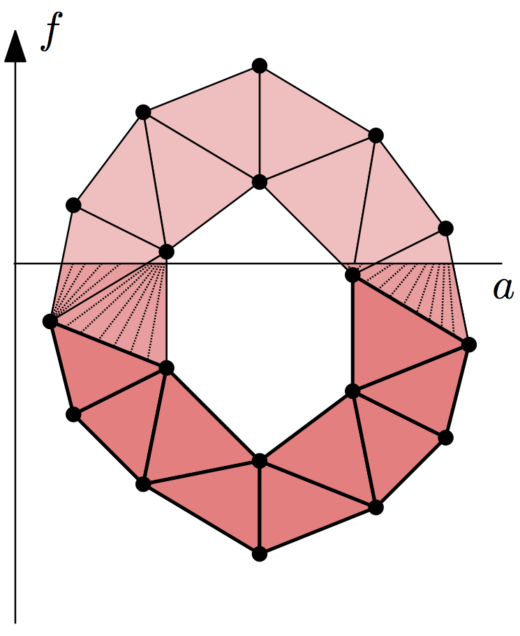
So given such a function \(f\), it suffices to assign to each simplex of
\(K\) the value of its maximum vertex. Sorting the resulting filtration
creates the lower-star filtration. To construct the symmetric upper-star
filtration, assign the minimum of the vertices as the simplex data and pass
reverse = True to sort().
Dionysus provides a helper function,
fill_freudenthal(), to build lower-star and
upper-star filtrations of the Freudenthal triangulation on a grid, with values given in a NumPy array.
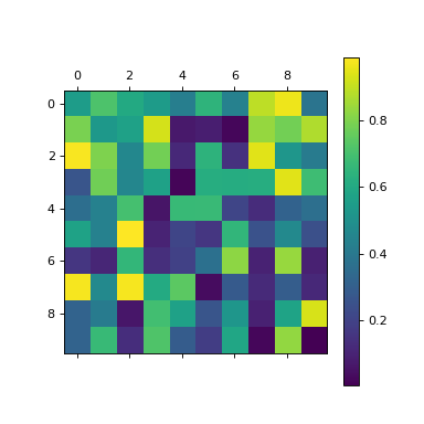
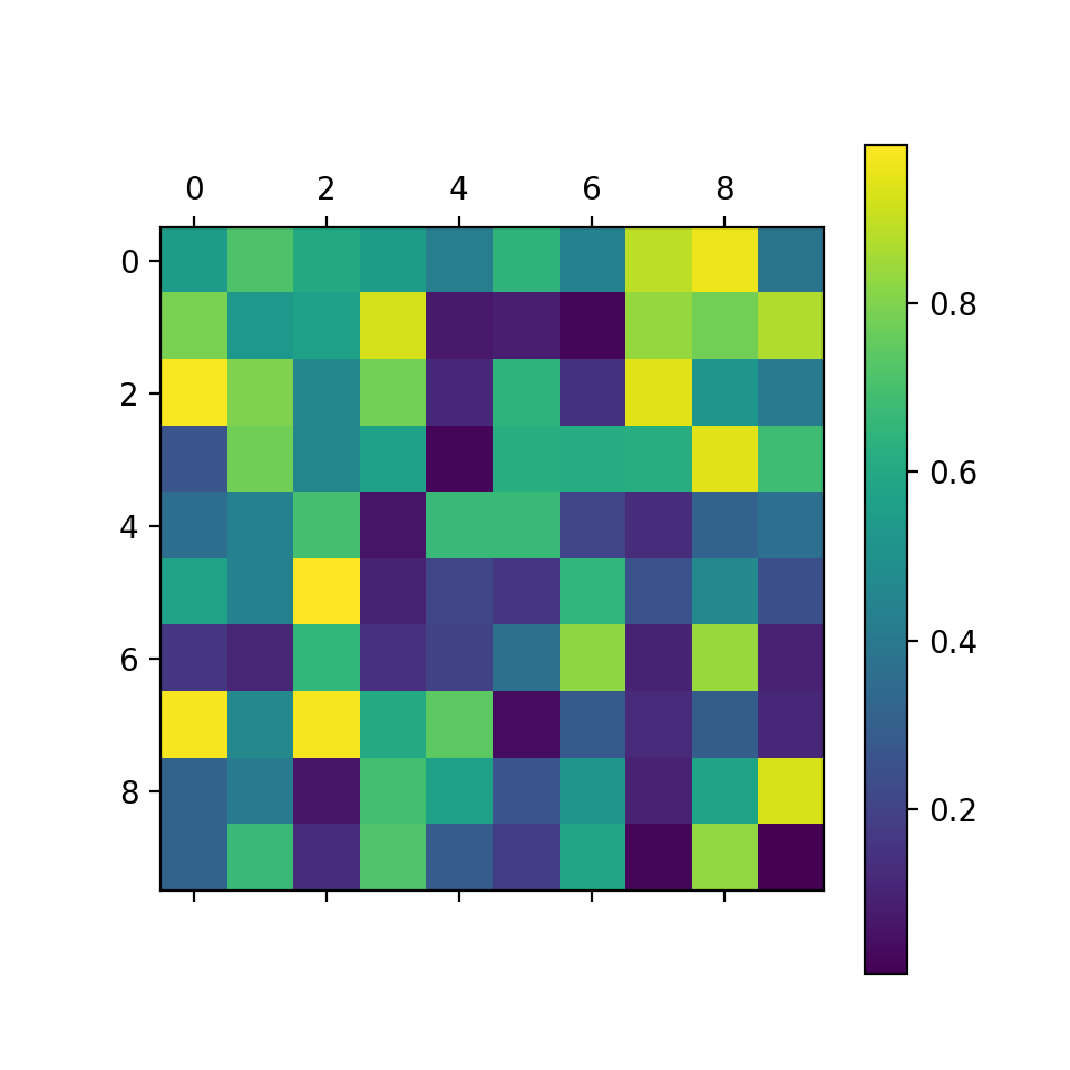
Take a random NumPy array:
>>> a = np.random.random((10,10))
>>> plt.matshow(a)
<...>
>>> plt.colorbar()
<...>

Use fill_freudenthal() to construct the triangulation:
>>> f_lower_star = d.fill_freudenthal(a)
>>> f_upper_star = d.fill_freudenthal(a, reverse = True)
Compute persistence as usual:
>>> p = d.homology_persistence(f_lower_star)
>>> dgms = d.init_diagrams(p, f_lower_star)
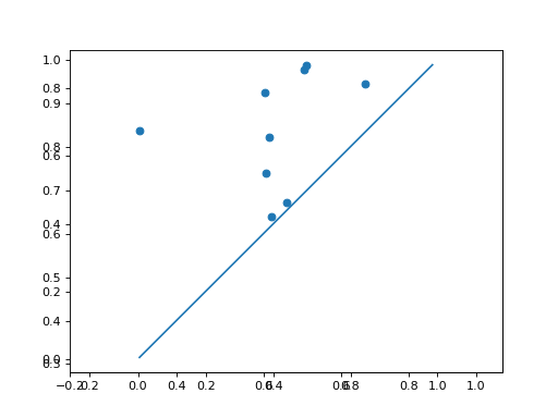
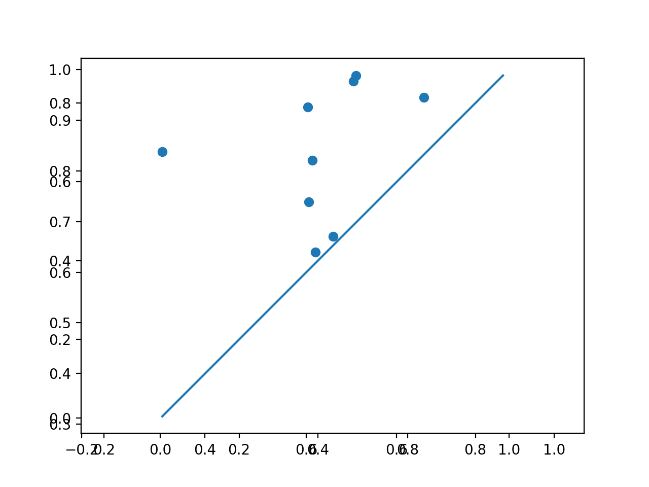
Use Plotting functionality to plot the diagrams:
>>> d.plot.plot_diagram(dgms[0])
>>> d.plot.plot_diagram(dgms[1])